
The most common way people invest is with strategic asset allocations to stocks and bonds, with perhaps a small allocation to alternatives. This approach passes for prudent diversification but is sub-optimal nonetheless. It is what Warren Buffett had in mind when he said diversification makes little sense if you know what you are doing. You may have less volatility than investing only in the stock market. But the cost of this approach is lower returns and less accumulated wealth. A better approach is to be in markets with a positive trend. This way, you can avoid performance drag caused by lagging assets.
My last article showed in more detail the advantages of trend following. It also discussed overcoming possible pitfalls, such as data overfitting. This article will detail how to better evaluate trend-following strategies and combine them into optimal portfolios.
What to Do and Not Do
A little over 5 years ago, some folks raised over $50 million for an ETF using the dual momentum ideas in my book. Their main change to my book’s Global Equities Momentum (GEM) model was their use of hundreds of correlated lookback periods.
I pointed out in a blog post and on my website’s FAQ page that this was unnecessary and my book’s simple GEM model would likely outperform this ETF. Since then, my GEM model has had more than twice the return of that ETF.
I also pointed out that adding different trading approaches rather than excessive lookback periods would be better. That is what I have been doing for the past 10 years.
It is not easy to come up with good trading methods. Specification biases and data overfitting are constant risks. We avoid that by rigorous robustness checks and simple approaches that have worked well over long out-of-sample periods. Rate-of-change and channel breakouts are two such methods as per my last article.
But we must still determine if our approaches are good enough to put in place. Most people look first at returns. The compound annual growth rate (CAGR) is a way to do that. The CAGR is actually a risk-adjusted but aggressive metric. If you have two strategies with the same annual return, the less volatile one will have a higher CAGR. But the CAGR doesn’t tell us much about our downside risk exposure.
So many also look at the maximum drawdown. But that is only one point in time. It doesn’t tell you about the frequency of drawdowns or their distribution. Maximum drawdowns are also time-dependent. The more data you have, the greater the chance for more significant maximum drawdowns.
The most common way of evaluating performance is the Sharpe ratio. This metric divides return, less the risk-free return, by the standard deviation of returns. This conveniently combines returns with a measure of volatility. Both academics and practitioners look at Sharp ratios.
One reason may be that Bill Sharpe, a Nobel laureate, created it. Another reason is you can draw statistical inferences using means and standard deviations. But these are not highly accurate unless returns are normally distributed. That’s not the case with financial assets. These often have negative skewness, while trend-following systems often have positive skewness. Skewness is a measure of extreme events at the tail ends of distributions. Some approaches with high Sharpe ratios can be vulnerable to catastrophic loss.
Alternative Reward-to-Risk Metrics
The Sortino ratio is a somewhat better but lesser-used performance metric to measure downside risk. It considers only volatility below the mean. However, it does not account for other areas of the distribution, such as fat tails or the desirability of positive skewness above the mean. Like the Sharpe ratio, it does not account for serial correlation in your results.
Another approach is to calculate a Sharpe ratio that accounts for higher moments of a distribution. You can find information on that here, here, here, and here. We look at skewness-adjusted Sharpe ratios but don’t usually include them in our presentations since they are not well known.
An alternative risk-adjusted measure is to divide the average exceeds return by the Value at Risk (VaR), which estimates probabilistic extreme risk exposure. We prefer to use the Ulcer Index (UI) instead since UI accounts for the duration and depth of all drawdowns. You get the Ulcer Performance Index (UPI) using the same logic as the Sharpe ratio by dividing excess return by the Ulcer Index. If I had to choose only one measure to look at, the UPI would be it. But it makes more sense to look at other things as well. It should be like looking at regression results, where you examine multiple numbers but also look at a plot of the residuals to identify issues that may not appear in the numbers.
Besides UPI, I consider skewness-adjusted Sharpe ratio, maximum drawdown, CAGR, and a visual examination of the results curve. You want to see consistency and little or no falloff in recent performance.
Portfolio Formation

Now that we know how to evaluate system performance and select attractive assets and trading approaches, we must know how to combine them. We want to select assets or approaches with low-to-moderate correlations. This can reduce portfolio volatility and drawdowns without reducing the average expected return.
In the 1950s, Harry Markowitz did seminal work on portfolio optimization called mean-variance optimization (MVO). He used returns, volatilities, and correlations to form “efficient portfolios” offering the highest expected return at different risk levels, or the lowest risk at various levels of expected return.
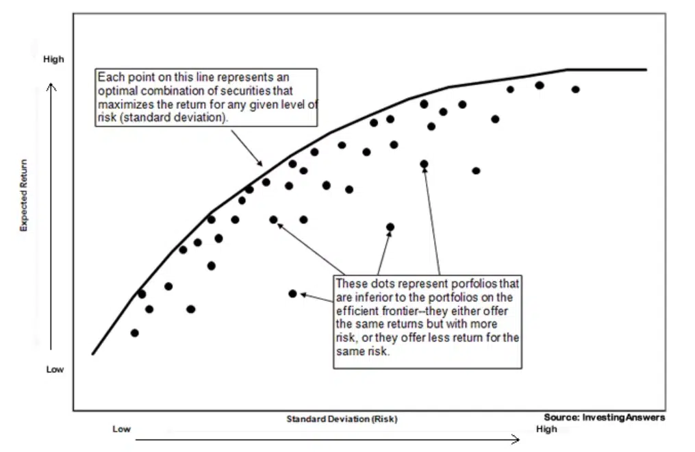
MVO is elegant and sounds appealing. But like some other attractive financial concepts, it doesn’t work well in practice. The inputs, especially returns, are unstable, and estimation errors multiply during optimization.
When we built our own MVO model in the 1980s, we found the outputs would jump around too much to be of practical use. We ended up using other information along with MVO.
In 2009, a research study showed that a simple equal-weight portfolio outperformed MVO going forward. Equal weighting is optimal if you have little or no information, but we have the information we discussed earlier.
Our approach begins by equal weighting our best systems, preferably those with low to moderate correlations. We then incrementally adjust the allocation percentages up or down until we get the most attractive portfolios based on the above criteria. Portfolio construction can be just as important as model selection.
An Example
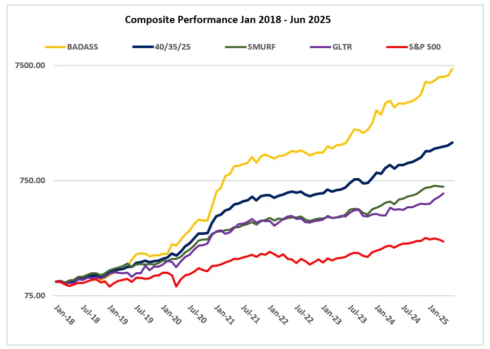
Here is an example of our three best proprietary models with low to moderate correlations. Combined portfolios are in the order of SMURF, BADASS, and GLTR. Performance is from January 2018 through June 2025. Real -time portfolio performance since January 2024, when we went public with BADASS and GLTR, has been similar to these numbers.
| GLTR | BADASS | SMURF | 40/40/20 | 45/35/20 | 40/35/25 | |
| CAGR | 24.7 | 78.6 | 30.5 | 48.2 | 45.9 | 47.5 |
| STD DEV | 20.0 | 31.6 | 13.5 | 17.6 | 16.7 | 16.6 |
| SHARPE | 1.20 | 2.02 | 2.05 | 2.35 | 2.37 | 2.37 |
| ADJ SHARPE | 1.41 | 2.40 | 2.04 | 2.63 | 2.62 | 2.61 |
| UPI | 4.81 | 28.10 | 13.73 | 23.34 | 22.40 | 22.07 |
| MAX DD | -15.8 | -12.4 | -10.7 | -8.3 | -8.2 | -8.1 |
| AVG DD | -3.7 | -1.6 | -1.1 | -0.9 | -0.9 | -0.9 |
| W% MOS | 61 | 76 | 73 | 79 | 79 | 78 |
Results do not guarantee future success nor represent returns that any investor attained. Performance includes reinvestment of interest and dividends. See our Disclaimer page for more information.