
Tail risk is the probability that an asset performs far below or far above its average past performance. Tail risk is an investor’s worst enemy. Extreme market moves can lead to changes in our risk preferences and cause us to act based on emotion rather than reason. Investors tend to buy when they would be better off selling, and sell when they should be buying. Gregg Fisher of Quent Capital said, “We don’t have people with investment problems. We have investments with people problems.”
My experience in the 1980s managing hedge funds and for the past ten years working with proprietary models is that investors make poor decisions when swayed by short-term performance.
Peter Lynch managed Fidelity’s Magellan Fund from 1977 to 1990. During that time, the fund’s average annual return was an impressive 29% per year. But Lynch pointed out that the average investor in his fund made only 7% per year. Investors would flee the fund when it had a setback and get back in after missing the recovery.
Ken Heebner’s CGM Focus Fund was ranked the best stock fund of the decade from 2000 to 2010. Its average annual return was over 18%. According to Morningstar, the average investor in that fund lost 17% annually during that period.
Morningstar’s annual “Mind the Gap” shows the persistent gap between investor returns and the biggest funds’ total returns.
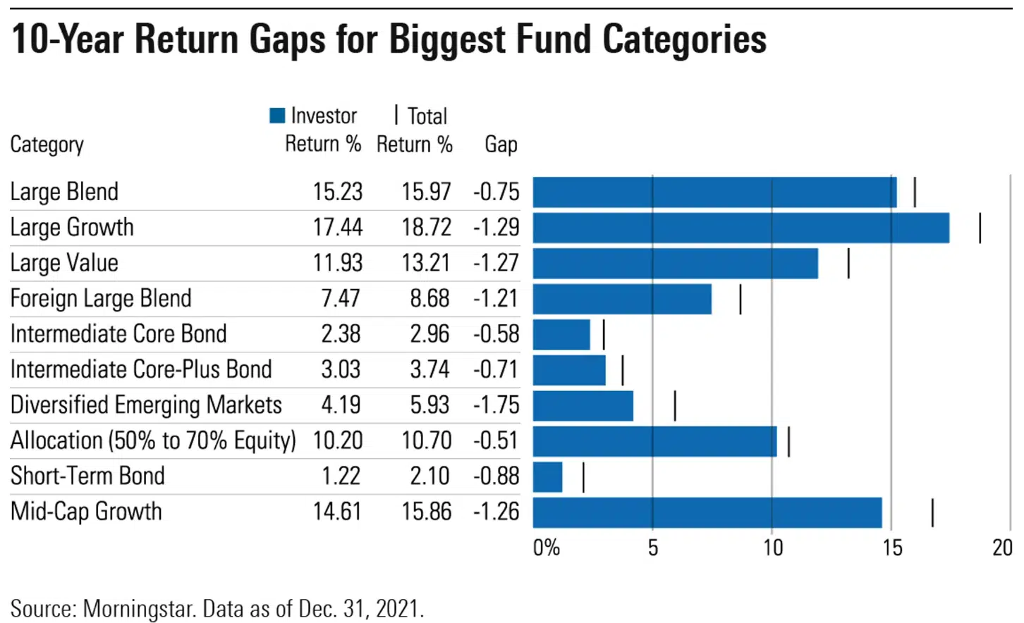
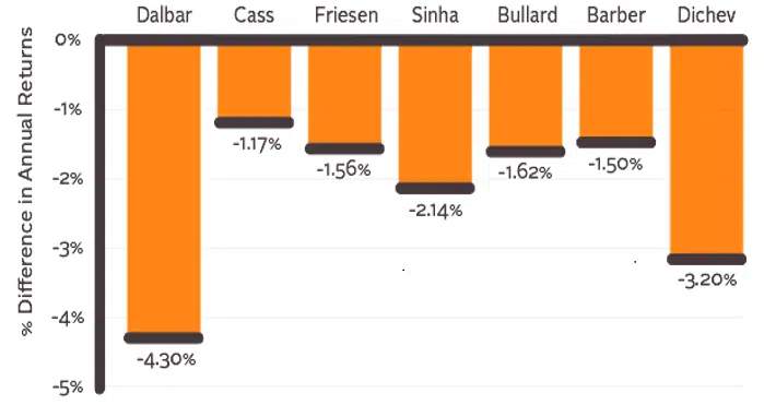
Other studies show similar results. Bad timing decisions by investors account for much of this underperformance. A reduction in return of 1 to 2% per year can mean substantially less terminal wealth.
Left Tail Risk
Left tail risk of extreme loss is especially problematic for those at or nearing retirement age. Their portfolios may not have time to recover from a 50% or greater drop in value. These investors especially need to protect themselves from left-tail risk.
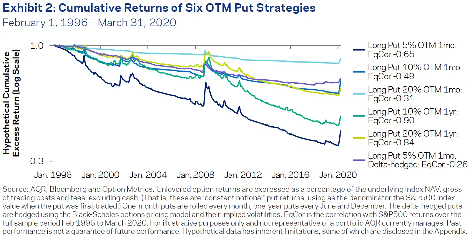
A direct way of managing left tail risk is to hedge by buying far out-of-the-money (OTM) puts. There are hedge funds and institutional money managers who offer this approach. But there are others, especially academics, who point to the high cost of hedging and the superiority of other approaches. AQR, for example, has several papers critical of put hedging [1]. But they may be comparing apples to oranges. AQR bases its analysis on 5% OTM puts, but practitioners usually use puts that are at least 20% OTM. This gives them larger positions and higher payoffs during severe bear markets.
This chart from AQR shows poor results with 5% OTM puts, which is what they use in their analysis. The best results here are with 20% OTM puts, which is in line with what successful practitioners use.
There are other ways to further improve the performance of put hedging. Mark Spitznagel, manager of a large tail-risk hedge fund, showed market outperformance of a 30% OTM tail-risk strategy from 1901 through 2013. This happened if they hedgd when the stock market was overvalued according to Tobin’s Q ratio [2].
Tail-risk manager Vineer Bhansali showed improved performance over a benchmark portfolio by liquidating 20% OTM hedges when they had a profit of 500% to 1000%. [3] My own research on a basket of ETFs confirms these results over the most recent 10-year period.
Even if tail-risk hedging creates a modest expense rather than a profit, it might be worth doing because of the protection it gives. A 50% drawdown requires a 100% gain to get even. Not having to make up those losses can lead to higher long-run returns. When you can mitigate left-tail risk, you may also be comfortable allocating more of your portfolio to equities. This can also lead to higher expected portfolio returns.
Drawbacks to Tail Risk Hedging
There are drawbacks one should keep in mind when considering tail-risk hedging. First is its accessibility. This is not usually a do-it-yourself project. There is only one retail fund manager, Aptus Capital Advisors, who uses tail-risk hedging with far OTM puts.
There is also some familiarity bias. Not that many investors are knowledgeable about tail risk hedging with puts.
Another drawback is tracking error. You might wait ten or more years underperforming by 1 to 3% annually until you can cash in on your hedges. Few investors can be that patient. CALPERS was using a well-known tail risk manager and dropped them before the 2020 market crash. This reportedly cost them over $1 billion in missed profits. Institutional investors may face career risk when they underperform their peers for more than a few years.
Diversification
A more accessible and popular way to deal with tail risk is diversification into assets that are not highly correlated to the stock market. Bonds are often used this way. But there are issues with this. First, other assets like bonds have a lower risk premium than stocks and so lower expected returns. Diversification with bonds can create a drag on long-term portfolio performance.
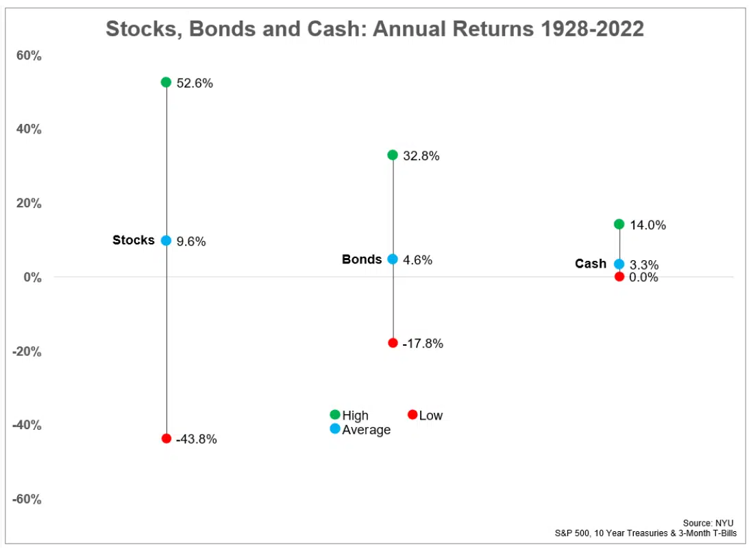
Second, bonds are not always uncorrelated to stocks.
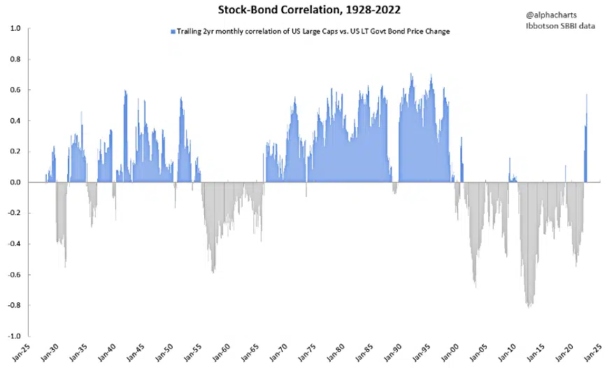
In 2022 when the S&P 500 was down 18.6, 10-Year Treasuries lost 15.6%. This was not the first time both markets have together come under pressure.
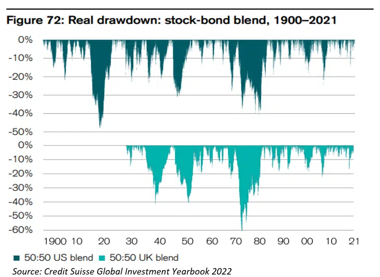
Some say that the only thing that goes up during a crisis is correlation. Under financial stress, investors tend to exit all risky assets. Bond diversification may not be effective in providing tail-risk protection when it is needed the most.
Trend
Our research agrees with others who have identified trend-following as the best way to deal with tail risk.
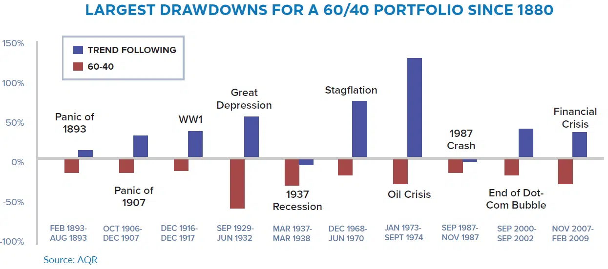
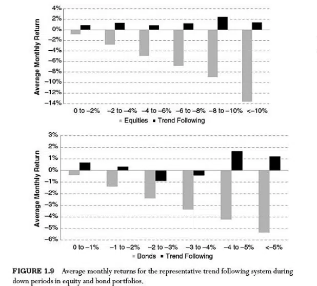
Greyserman and Kaminski use a simple form of trend following by holding assets only when they have a positive return over the past 12 months. This is similar to absolute momentum as explained in my book. Trend applied this way to stock and bond indices since 1695 and 1300 led to much higher returns than buy-and-hold.
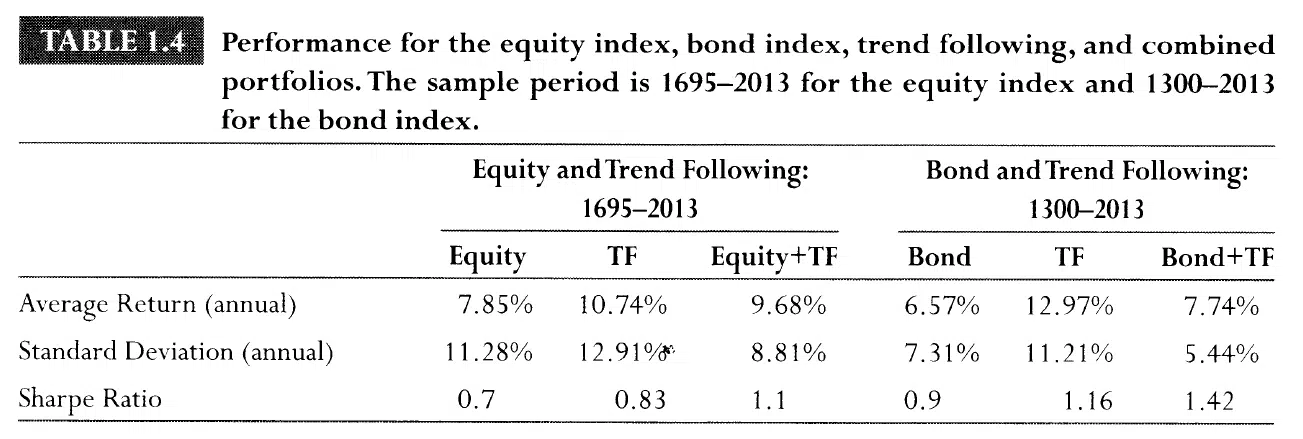
Risk exposure, especially left-tail risk, was also reduced during down periods, according to the authors.
Yet few investors are willing to apply trend following to their entire portfolio. Most have a strong buy-and-hold bias toward stocks and bonds. They often have limited familiarity with and confidence in trend.
Managed Futures
Until recent years, both academics and practitioners regarded trend following as something akin to voodoo. Many of those who are now more receptive to trend think of it as an “alternative” investment worthy of only a small portfolio allocation.
Along those lines, trend often gets equated with managed futures. These are considered high risk because of their leverage and the volatility of commodities, even though their drawdowns are often no greater than those of the stock market. Because of this and the familiarity bias of investors, managed futures managers themselves often promote their programs as minor allocations to a balanced portfolio.
The Mount Lucas Management (MLM) managed futures program goes back to January 1988. There are other managed futures programs that have also been around since the 1980s or 1970s. These include Dunn, Campbell, Chesapeake, Milburn, and EMC. MLM is typical of these and has available index data. It is also easily accessible through the KMLM ETF.
Like bonds, managed futures are accessible through ETFs and mutual funds. But managed futures offer some advantages over bonds as a portfolio diversifier. First, managed futures can be long or short. This allows them to better adapt to changing market conditions,
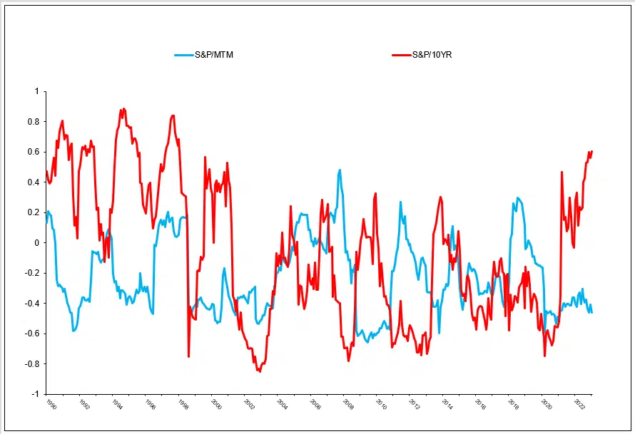
Managed futures are also less correlated to the stock market. The correlation of MLM monthly returns to the S&P 500 is -0.27, while the correlation of 10-year U.S. Treasury bonds to the S&P 500 is -.03. MLM correlations are also more stable than stock/bond correlations.
Monthly Correlations January 1988 through January 2023
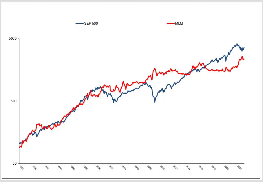
Here is the MLM index from its start in January 1988 along with the S&P 500 index. We can see the negative correlation and potential benefit of diversification in smoothing volatility and reducing the left tail risk of the stock market.
Here is a 60% allocation to the S&P 500 and a 40% allocation to the MLM index compared to a 60/40 allocation to the S&P 500 and 10-year Treasury bonds. The Sharpe ratio of the 60/40 MLM portfolio is 0.71 versus 0.56 for the stock and bond 60/40 portfolio.
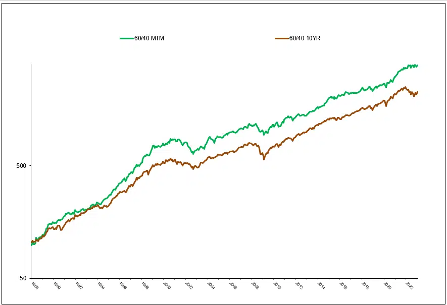
The results are hypothetical results and are NOT an indicator of future results and do NOT represent returns that any investor actually attained. Indexes are unmanaged and do not reflect management or trading fees, and one cannot invest directly in an index.
Issues with Managed Futures
The first obstacle in using managed futures is familiarity bias as mentioned earlier. Next is survivorship risk. Arnold & Zaffaroni found an 11.1% failure rate among Commodity Trading Advisors from 1994 through 2009. They noted that larger, systematic advisors have the highest chance of survival. But that is not always the case.
One of the largest and most successful systematic advisors was John W. Henry & Company. They managed $2.5 billion in assets in 2006 yet went out of business in 2012 due to poor performance.
Another drawback to having an allocation to managed futures is long periods of tracking error. From 2009 through 2021, MTM’s performance was flat. This would have created an extended drag on portfolio performance. While negative correlation can reduce portfolio drawdowns, it can also reduce gains during bull markets.
We incorporate managed futures into some of our models. But we only use them when their aggregate trend and relative strength are positive according to dual momentum.
Bonds Revisited
Our research shows that trend following is highly effective when applied to the fixed-income market. This fact does not get the attention that it deserves.
Trend-following with bonds does not have most of the issues associated with tail-risk hedging and managed futures. Familiarity is not a problem since investors are used to large fixed-income allocations. If constructed well, one need not worry about bond portfolios going out of business.
High-yield bonds move with the stock market. Using relative strength and trend (dual momentum) to rotate into high-yield bonds, tracking error should not be as much of an issue with bonds.
Dual Momentum Fixed Income (DMFI)
Dual Momentum Fixed Income is our simplest and oldest proprietary dual momentum model. Those who have read my book should be able to come up with their own version of a dual momentum bond model.
DMFI applies relative strength and trend to short and intermediate-term bonds. Compared to long-term bonds, intermediate bonds have a premium because of the reinvestment risk when these bonds become due. We gladly capture that premium. We do not care about reinvestment risk since we base our buy and sell decisions on relative strength and trend. Here are the DMFI results since 1970 when there was enough bond data to be meaningful.
Dual Momentum Fixed Income Performance – Jan 1970 through Mar 2023
DMFI | 10 YR | S&P 500 | 60/40 | 60/40 DMFI | |
CAGR | 8.0 | 7.2 | 9.3 | 9.5 | 11.3 |
Standard Deviation | 5.6 | 8.0 | 17.9 | 10.2 | 11.5 |
Sharpe Ratio | 1.38 | 0.34 | 0.59 | 0.50 | 0.82 |
Ulcer Index | 1.87 | 3.99 | 13.70 | 5.90 | 3.80 |
Worst Drawdown | -6.3 | -21.0 | -52.9 | -29.7 | -16.3 |
Avg Drawdown | -1.1 | -2.3 | -7.5 | -3.2 | -2.1 |
% Up Months | 71 | 60 | 66 | 64 | 66 |
Results do not guarantee future success and do not represent returns that any investor attained. You cannot invest directly in our models. 10 YR is the ICE U.S. Treasury 7-10 Year Bond Index. 60/40 is 60% S&P 500 and 40% ICE U.S. Treasury 7-10 Year Bond Index. 60/40 DMFI is 60% S&P 500 and 40% DMFI. CAGR is the compound annual growth rate. Drawdowns are on a month-end basis. Ulcer Index measures the depth and duration of drawdowns from earlier highs. See our Disclaimer page for more disclosures.
DMFI is an attractive alternative for those wanting to hold a balanced stock and bond portfolio. Substituting DMFI for intermediate bonds in a 60/40 stock/bond portfolio would have boosted returns by 180 bps annually while reducing the worst portfolio drawdown.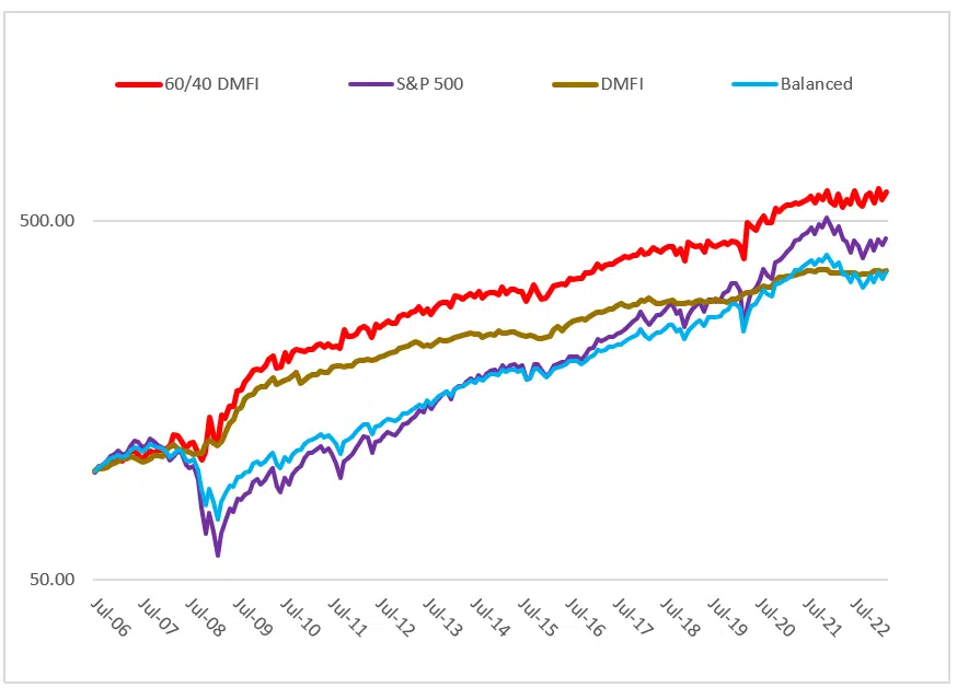 Results are hypothetical results and are NOT an indicator of future results and do NOT represent returns that any investor actually attained. Indexes are unmanaged and do not reflect management or trading fees, and one cannot invest directly in an index.
A Barbell Approach
Another way to use DMFI is to combine it with our aggressive NASDAQ Breadth & Trend (QBAT) model in a “barbell strategy” as advocated by Nassim Taleb. As he describes it, “If you know that you are vulnerable to prediction errors, and if you accept that most ‘risk measures’ are flawed…then your strategy is to be as hyper-conservative and hyper-aggressive as you can be…”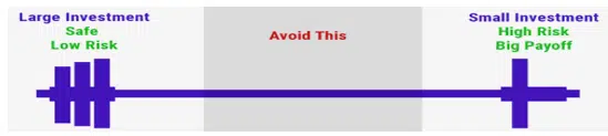 QBAT is our most aggressive model. It uses breadth with dual momentum and mean reversion. Each of these adds incremental value not captured by the other approaches. [4]
QBAT can hold a 2X leveraged ETF when all conditions warrant it [5]. QBAT’s aggressiveness matches up well with DMFI, our most conservative model.
Underperformance Risk of Trend Following
Trend following can be effective in dealing with left-tail risk. But there can be false signals causing returns to lag their benchmarks during strong and prolonged bull markets. It is during bear markets that trend following adds the most value.
When missing out on larger bull market returns, investors may lose sight of the big picture and grow impatient. My experience shows more investors abandoning trend-following because of impatience than for any other reason. Warren Buffett once said the stock market is a mechanism to transfer wealth from the impatient to the patient.
QBAT addresses this issue head-on. Unlike other trend-based models, the model QBAT has done well in all market environments.
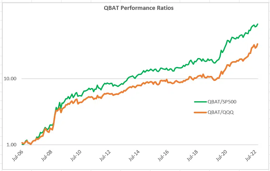
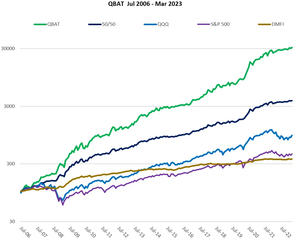
Here are some allocations combining QBAT and DMFI ranging from 70%/30% to 20%/80%. Even modest allocations to QBAT can have a meaningful impact on portfolio performance.
QBAT with DMFI August 2006 through March 2023
QBAT | DMFI | 60/40 | 50/50 | 40/60 | 30/70 | 20/80 | 10/90 | |
CAGR | 40.7 | 8.0 | 27.3 | 24.2 | 20.9 | 17.6 | 14.4 | 11.1 |
STD DEV | 23.8 | 5.6 | 15.4 | 13.4 | 11.4 | 9.5 | 7.8 | 6.5 |
SHARPE | 1.57 | 1.38 | 1.66 | 1.69 | 1.73 | 1.76 | 1.76 | 1.67 |
ULCER IDX | 4.45 | 1.87 | 2.77 | 2.38 | 2.02 | 1.71 | 1.37 | 1.24 |
MAX DD | -19.6 | -6.3 | -12.8 | -11.1 | -9.6 | -8.1 | -8.5 | -7.1 |
AVG DD | -2.3 | -1.1 | -1.4 | -1.2 | -1.0 | -0.9 | -0.5 | -0.5 |
W% MOS | 68 | 72 | 68 | 70 | 70 | 70 | 76 | 78 |
Results do not guarantee future success and do not represent returns that any investor attained. Performance includes reinvestment of interest and dividends. Positions are rebalanced monthly. CAGR is the compound annual growth rate. Maximum drawdown is on a cumulative month-end basis. Ulcer Index measures the depth and duration of drawdowns from earlier highs. Leveraged ETFs have high risk and extreme volatility. See the Disclaimer at the end of this document for more information.
Contact us if you would like fact sheets or more information about our proprietary models.
Conclusion
Tail risk is an investor’s worst enemy (other than him or herself). Put hedging can be effective in mitigating left tail risk if it is done the right way. But there are drawbacks to that approach. These include accessibility and long periods of benchmark underperformance.
Diversification alone may not be effective during periods of market stress when you need it the most. Investors tend to abandon all risky assets when faced with severe market stress. Diversifying assets also have lower expected returns than stocks and thus create a drag on portfolio performance.
Managed futures are adaptable by going long or short. But most investors would not be comfortable having an allocation to managed futures that is large enough to be meaningful. Like put hedging, managed futures are subject to familiarity bias and long periods of underperformance.
Trend applied to a mix of diversified sectors of the bond market may be the best solution for dealing with left-tail risk. Bonds are familiar to everyone.
Dual momentum applied to bonds has had a low correlation to equities. This should make it useful for diversification and potential risk reduction in both balanced and aggressive portfolios.
[1] Israelov (2017), “The Elusive Benefits of Protective Puts”
Ilmanen, Thapar, Tummala, & Villalon (2020), “Tail Risk Hedging: Contrasting Put and Trend Strategies”
[2] Spitznagel (2013), The Dao of Capital: Austrian Investing in a Distorted World, John Wiley & Sons
[3] Bhansali (2014), Tail Risk Hedging: Creating Robust Portfolios for Volatile Markets, McGraw-Hill
Bhansali (2020), “Monetization Matters: Active Tail Risk Management and the Great Virus Crisis”
[4] For an example see, Zaremba et al. (2021), “Herding for Profits: Market Breadth and the Cross-Section of Global Equity Returns.”
[5] Long-only 2X leveraged ETFs work well without much volatility drag for holding periods of up to 1 year. See Lu, Wang, & Zhang (2009), “Long Term Performance of Leveraged ETFs” and Double Digit Numeric’s “The Long Term Behaviour of Leveraged ETFs.”1480